

What the $#@! is parallelism, anyhow?
We take inspiration from Amdahl's Law to give a more "authoritative" introduction to the basic concepts of multithreaded execution — work, span, and parallelism.

I’m constantly amazed how many seemingly well-educated computer technologists bandy about the word parallelism without really knowing what they’re talking about. I can’t tell you how many articles and books I’ve read on parallel computing that use the term over and over without ever defining it. Many of these “authoritative” sources cite Amdahl’s Law, originally proffered by Gene Amdahl in 1967, but they seem blissfully unaware of the more general and precise quantification of parallelism provided by theoretical computer science. Since the theory really isn’t all that hard, it’s curious that it isn’t better known. Maybe it needs a better name — “Law” sounds so authoritative. In this blog, I’ll give a brief introduction to this theory, which incidentally provides a foundation for the efficiency of the OpenCilk runtime system.
Amdahl’s Law
First, let’s look at Amdahl’s Law and see what it says and what it doesn’t say. Amdahl made what amounts to the following observation. Suppose that 50% of a computation can be parallelized and 50% can’t. Then, even if the 50% that is parallel took no time at all to execute, the total time is cut at most in half, leaving a speedup of less than 2. In general, if a fraction p of a computation can be run in parallel and the rest must run serially, Amdahl’s Law upper-bounds the speedup by 1/(1-p).
This argument was used in the 1970’s and 1980’s to argue that parallel computing, which was in its infancy back then, was a bad idea — the implication being that most applications have long, inherently serial subcomputations that limit speedup. We now know from numerous examples that there are plenty of applications that can be effectively sped up by parallel computers, but Amdahl’s Law doesn’t really help in understanding how much speedup you can expect from your application. After all, few applications can be decomposed so simply into just a serial part and a parallel part. Theory to the rescue!
A model for multithreaded execution
As with much of theoretical computer science, we need a model of multithreaded execution in order to give a precise definition of parallelism. We can use the dag model for multithreading. (A dag is a directed acyclic graph.) The dag model views the execution of a multithreaded program as a set of instructions (the vertices of the dag) with graph edges indicating dependencies between instructions. We say that an instruction x precedes an instruction y, sometimes denoted x≺y, if x must complete before y can begin. In a diagram for the dag, x≺y means that there is a positive-length path from x to y. If neither x≺y nor y≺x, we say the instructions are in parallel, denoted x∥y. The figure below illustrates a multithreaded dag that indicates, for example, 1≺2, 6≺12, and 4∥9.

Just by eyeballing, what would you guess is the parallelism of the dag? About 3? About 5? It turns out that two measures of the dag, called work and span, allow us to define parallelism precisely, as well as to provide some key bounds on performance. I’m going to christen these bounds “Laws,” so as to compete with the Amdahl cognoscenti.
Work
The first important measure is work, which is what you get when you add up the total amount of time for all the instructions. Assuming for simplicity that it takes unit time to execute an instruction, the work for the example dag is 18, because there are 18 vertices in the dag. The literature contains extensions to this theoretical model to handle nonunit instruction times, caching, etc., but for now, dealing with these other effects will only complicate matters.
Let’s adopt a simple notation. Let TP be the fastest possible execution time of the application on P processors. Since the work corresponds to the execution time on 1 processor, we denote it by T1. Among the reasons that work is an important measure is because it provides a bound — oops, I mean Law — on any P-processor execution time:
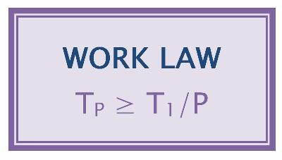
The Work Law holds, because in our model, each processor executes at most 1 instruction per unit time, and hence P processors can execute at most P instructions per unit time. Thus, to do all the work on P processors, it must take at least T1/P time.
We can interpret the Work Law in terms of speedup. Using our notation, the speedup on P processors is just T1/TP, which is how much faster the application runs on P processors than on 1 processor. Rewriting the Work Law, we obtain T1/TP ≤ P, which is to say that the speedup on P processors can be at most P. If the application obtains speedup proportional to P, we say that the speedup is linear. If it obtains speedup exactly P (which is the best we can do in our model), we say that the application exhibits perfect linear speedup. If the application obtains speedup greater than P (which can’t happen in our model due to the work bound, but can happen in models that incorporate caching and other processor effects), we say that the application exhibits superlinear speedup.
Span
The second important measure is span, which is the longest path of dependencies in the dag. The span of the dag in the figure is 9, which corresponds to the path 1→2→3→6→7→8→11→12→18. This path is sometimes called the critical path of the dag, and span is sometimes referred to in the literature as critical-path length or depth. Since the span is the theoretically fastest time the dag could be executed on a computer with an infinite number of processors (assuming no overheads for communication, scheduling, etc.), we denote it by T∞.
Like work, span also provides a bou…, uhhh, Law on P-processor execution time:
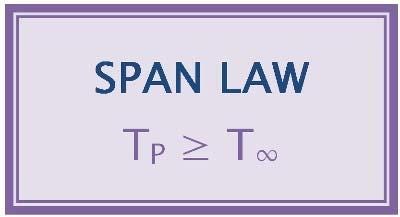
The Span Law holds for the simple reason that a finite number of processors cannot outperform an infinite number of processors, because the infinite-processor machine could just ignore all but P of its processors and mimic a P-processor machine exactly.
Parallelism
Parallelism is defined as the ratio of work to span, or T1/T∞. Why does this definition make sense? There are several ways to understand it:
The parallelism T1/T∞ is the average amount of work along each step of the critical path.
The parallelism T1/T∞ is the maximum possible speedup that can be obtained by any number of processors.
Perfect linear speedup cannot be obtained for any number of processors greater than the parallelism T1/T∞. To see this third point, suppose that P > T1/T∞, in which case the Span Law TP ≥ T∞ implies that the speedup satisfies T1/TP ≤ T1/T∞. Since the speedup is strictly less than P, it cannot be perfect linear speedup. Note also that if P ≫ T1/T∞, then T1/TP ≪ P — the more processors you have beyond the parallelism, the less “perfect” the speedup.
For our example, the parallelism is 18/9 = 2. Thus, no matter how many processors execute the program, the greatest speedup that can be attained is only 2, which frankly isn’t much. Somehow, to my eye, it looks like more, but the math doesn’t lie.
Amdahl’s Law Redux
Amdahl’s Law for the case where a fraction p of the application is parallel and a fraction 1-p is serial simply amounts to the special case where T∞ > (1-p)T1. In this case, the maximum possible speedup is T1/T∞ < 1/(1-p). Amdahl’s Law is simple, but the Work and Span Laws are far more powerful.
In particular, the theory of work and span has led to an excellent understanding of multithreaded scheduling, at least for those who know the theory. As it turns out, scheduling a multithreaded computation to achieve optimal performance is NP-complete, which in lay terms means that it is computationally intractable. Nevertheless, practical scheduling algorithms exist based on work and span that can schedule any multithreaded computation near optimally. The OpenCilk runtime system contains such a near-optimal scheduler. We’ll talk about multithreaded scheduling in a future post, where we’ll see how the Work and Span Laws really come into play.
[This work is derived from Cilk Plus documentation with permission of Intel Corporation and Cilk Arts.]
Fastcode is dedicated to all of software performance engineering (SPE)
Techniques of SPE include parallelism, vectorization, caching, algorithms, data structuring, compiler optimization, and more.
Tools of SPE include high-resolution timers, performance profilers, memory analyzers, scalability analyzers, race detectors, and more.
Theoretical foundations of SPE include task-parallel scheduling, work/span analysis, reuse distance, cache-oblivious algorithms, data structures, and more.
Let’s make SPE easier for everyone
What do you think is interesting right now about SPE? Why does it matter? If you have an idea for an SPE story, please let us know.